From a Probabilistic Perspective

Tags: optimization, LP

Useful links:

https://sites.math.washington.edu/~rothvoss/lecturenotes/lasserresurvey.pdf
https://web.stanford.edu/class/cs369h/
Laurent’s survey [1]
https://rameesh-paul.github.io/sos.pdf
https://www.ams.jhu.edu/~abasu9/papers/main-Lasserre.pdf
Chapter 3 of Ali Kemal Sinop’s PhD thesis

When I started writing this post, I hadn’t found so many “useful links” yet. The content below and link 1.2. only focus on using the Lasserre hierarchy on LPs, while 3.4.5.6. mention more general cases.

1 $K\subset [0,1]^n \to K\cap \{0,1\}^n$

We want to solve a 0-1 integer program. Since this task is NP-hard in general, we usually consider its linear relaxation. Different LP formulations have different integrality gaps. For example, consider the following linear relaxation of the max matching IP in non-bipartite graph.

\begin{aligned} \sum_{e\in \delta(v)} x(e)&\leq 1 & &\forall v\in V\\ x(e)&\in [0,1] & &\forall e\in E \end{aligned}

:(, this polytope is not integral. Edmonds proved that the following formulation is integral.

\begin{aligned} \sum_{e\in \delta(v)} x(e)&\leq 1 & &\forall v\in V\\ x(e)&\in [0,1] & &\forall e\in E\\ \sum_{e\in E[U]} x(e) &\leq (|U|-1)/2 & &\forall U\subset V, |U| \text{ odd} \end{aligned}

Schrijver [2] showed that those odd constraints can be obtained by adding cutting planes to the previous polytope. Fortunately for matching polytope we have a polynomial time separation oracle. However, for harder problems adding cutting planes may make the program NP-hard to solve. Lasserre hierarchy is a method to strengthen the polytope to approaching the integer hull while providing provable good properties and keeping the program polynomial time solvable (if applied constant number of times).

2 Probability Perspective

There is a good interpretation of the linear relaxation of 0-1 integer programs. Let

K=\left\{ x\in \mathbb{R}^n| Ax\geq b \right\}\subset [0,1]^n

be the polytope of the linear relaxation. The goal of solving the integer program is to describe all possible discrete distribution over

K\cap \left\{ 0,1 \right\}^n

. Note that for a fixed distribution the expected position

(\sum_p \mathop{\mathrm{Pr}}[X_p(1)=1] x_p(1),...,\sum_p \mathop{\mathrm{Pr}}[X_p(n)=1] x_p(n))^T

is in

\mathop{\mathrm{conv}}(K\cup \left\{ 0,1 \right\}^n)

and iterating over all possible distribution gives us the integer-hull. Hence we can find the integral optimal solution if having access to all distribution over integer points.

For any

x\in K

x_i

can be seen as the probability of

x_i=1

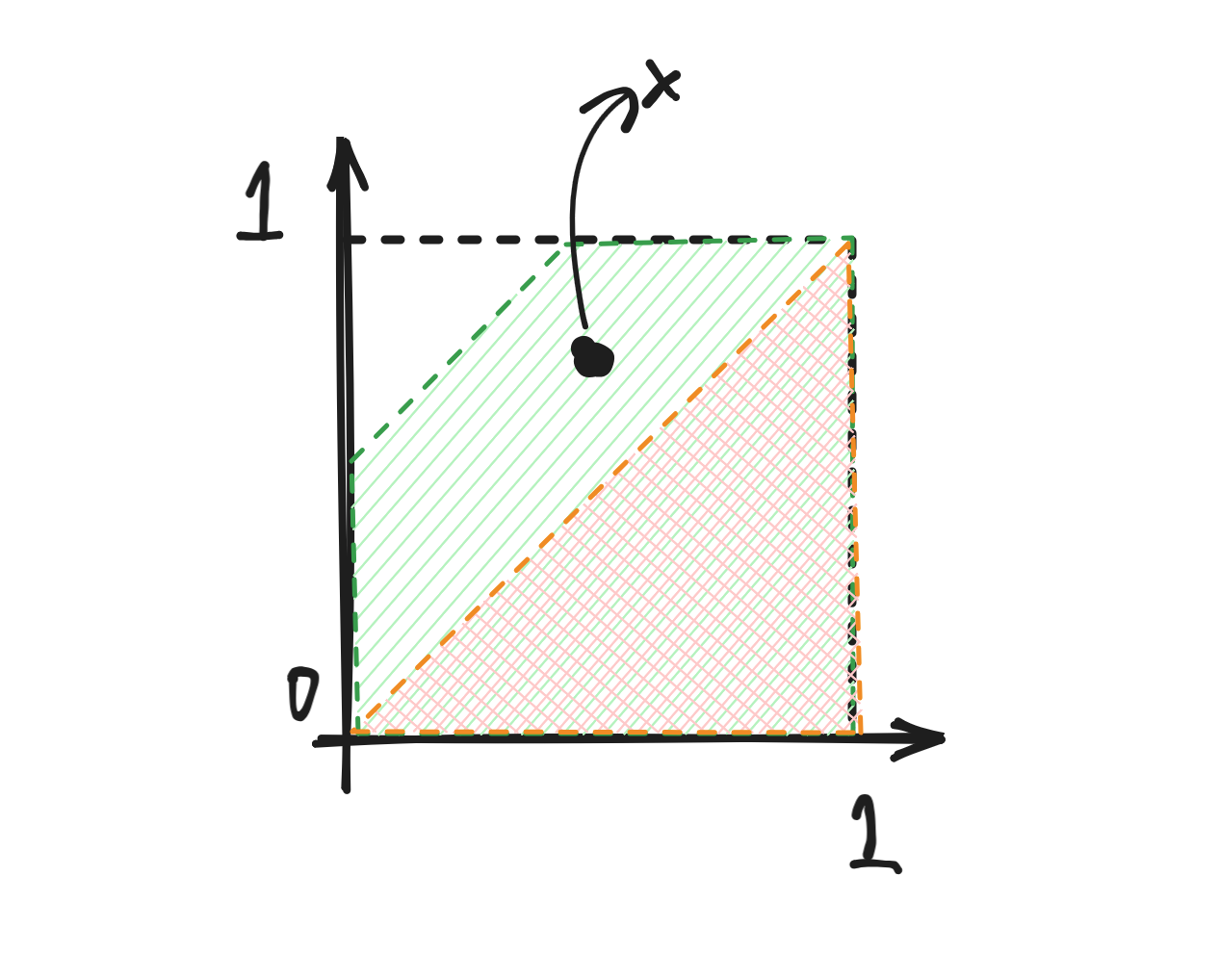
. We only care about the discrete distribution on feasible integral points. However, each

x\in K

only describes some marginal probabilities and this this marginal probability may not be even feasible. Consider the following 2D example. Any point in

\text{green area}\setminus \text{orange area}

is not a marginal distribution of any possible joint distribution over

(0,0),(1,0)

and

(1,1)

. The idea is to iteratively prune this area.

Now we need to think about how to represent all possible joint distribution. One natural way is to use a vector

y\in \mathbb{R}^{2^n}

for the distribution law of every possible integer point in

\left\{ 0,1 \right\}^n

. However, this method does not work well with our existing marginal probabilities. Let

y\in \mathbb{R}^{2^{n}}

be a random vector such that

y_I=\mathop{\mathrm{Pr}}[\bigwedge_{i\in I}(x_i=1)]

and

y_\emptyset=1

. Computing all feasible

y

is the same as finding all possible bivariate discrete distribution on the integer points. To make

y

a feasible probability from some joint distribution and to make

(y_{\left\{ 1 \right\}},...,y_{\left\{ n \right\}})^T\in K

we have to add more constraints.

2.1 Feasible Probability

For now let’s forget about

K

and consider

y\in [0,1]^{2^{[n]}}

and a discrete distribution

D

\left\{ 0,1 \right\}^n

. We want to make

y_I=\mathop{\mathrm{Pr}}_{D}[\bigwedge_{i\in I}(X_i=1)]

. In fact, there is a one to one correspondence between

y

and

D

. If

D

is given, computing

y_I

is easy for any

I\subseteq [n]

. If

y

is given, recovering the distribution

D

is the same as solving a system of

2^n

linear equations with

2^n

variables (

2^n-1

of the the equations come form

y_I

, and the remaining one is

\sum_p D(p)=1

.) Thus, with a slight abuse of notation, we will refer to

y

as a distribution.

We work with the 2D example first. Let

x=(x_1,x_2)^T\in K

be a marginal distribution. One can see that

y=(1,x_1,x_2,\mathop{\mathrm{Pr}}[X_1=X_2=1])^T

and the last number is not arbitrary. In fact,

\mathop{\mathrm{Pr}}[X_1=X_2=1]

must in range

[\max(0, x_1+x_2-1),\min(x_1,x_2)]

To make sure

y

is indeed a probability distribution the moment matrix is considered. The moment matrix

M(y)

is of size

2^n \times 2^n

and

M(y)[I,J]

is defined as the expectation

E[\prod_{i\in I\cup J}X_i]=y_{I\cup J}

(the only non-zero term is

1\cdot \mathop{\mathrm{Pr}}[\bigwedge_{i\in I\cup j}(X_i=1)]=y_{I\cup J}

). The expectation is taken over the distribution defined by

y

Lemma1

For any probability distribution

y

, the moment matrix is psd.

Proof

We need to verify

z^T M(y) z\geq 0

for any

z

\begin{aligned} z^T M(y) z &= \sum_I \sum_J z_I y_{I\cup J} z_J\\ &= \sum_I \sum_J z_I E[\prod_{i\in I\cup J} X_i] z_J\\ &= E\left[\left( \sum_I (z_I \prod_{i\in I} X_i)\right)^2 \right] \end{aligned}

Note that in the proof something like sum of squares appears. Lasserre hierarchy has deep connections with SOS optimization and is also known as sum-of-squares hierarchy.

Lemma2

M(y)

is psd then

y

is a probability distribution.

It is easy to see that

y_I\in [0,1]

for all

I\subseteq [n]

. Consider the following submatrix

\begin{bmatrix} \emptyset & y_I\\ y_I & y_I \end{bmatrix}

It is psd since

M(y)

is psd. The determinant is

y_I(1-y_I)\geq 0

Let

\mathop{\mathrm{Pr}}_D[p]

be the probability of selecting

p\in\left\{ 0,1 \right\}^n

D

. It remains to prove the following system of linear equations has a solution such that

\mathop{\mathrm{Pr}}_D[p]\in [0,1]

for all

p

\begin{aligned} y_{[n]} &= \mathop{\mathrm{Pr}}_D[\mathbf 1]\\ y_{[n]\setminus \left\{ n \right\}} &= \sum_{p:\bigwedge\limits_{i\in [n-1]}(p_i=1)} \mathop{\mathrm{Pr}}_D[p]\\ y_{[n]\setminus \left\{ n-1 \right\}} &= \sum_{p:\bigwedge\limits_{i\in [n]\setminus \left\{ n-1 \right\}}(p_i=1)} \mathop{\mathrm{Pr}}_D[p]\\ &\vdots \\ y_{\left\{ 1 \right\}} &= \sum_{p:p_1=1} \mathop{\mathrm{Pr}}_D[p]\\ y_\emptyset &= \sum_p \mathop{\mathrm{Pr}}_D[p] \end{aligned}

I believe this can be proven with the idea of Lemma 2 here.

2.2 Projection in $K$

Let the projection of

y

(y_{\left\{ 1 \right\}},\dots,y_{\left\{ n \right\}})^T

. For any

y

the projection should always lie in

K

. One may want to define moment matrices for constraints

Ax\geq b

. This is called the moment matrix of slacks. For simplicity we only consider one linear constraint

a^Tx-b\geq 0

. The moment matrix for this constraint is

M(y)=\left( \sum_{i=1}^n a_i y_{I\cup J\cup \left\{ i \right\}}-b y_{I\cup J} \right)_{I,J\subseteq [n]}

. Then we can do similar arguments.

\begin{aligned} z^T M(y) z &= \sum_I \sum_J z_I z_J (\sum_{i=1}^n a_i y_{I\cup J\cup \left\{ i \right\}}-b y_{I\cup J})\\ &= \sum_I \sum_J z_I z_J (\sum_i a_i E[\prod_{k\in I\cup J\cup\left\{ i \right\}} X_k] - b E[\prod_{k\in I\cup J}X_k] )\\ &= E\left[ \sum_I \sum_J z_I z_J (\sum_i a_i X_i -b) \prod_{k\in I\cup J}X_k \right]\\ &= E\left[ (\sum_i a_i X_i -b) \left(\sum_I z_I \prod_{i\in I} X_i \right)^2 \right] \end{aligned}

Note that we can combine the expectations since they are taken over the same probability distribution. Now assume that we have

a^TX-b\geq 0

\begin{aligned} E&\left[ (\sum_i a_i X_i -b) \left(\sum_I z_I \prod_{i\in I} X_i \right)^2 \right]\\ &= \sum \mathop{\mathrm{Pr}}[\cdots](a^T X-b)\left(\sum_I z_I \prod_{i\in I} X_i \right)^2 \geq 0 \end{aligned}

a^TX\geq b

is satisfied, then the corresponding slack moment matrix is psd.

Finally, this is a more formal definiton.

Definition3

t

-th level of Lasserre hierarchy

The

t

-th level of Lasserre hierarchy

\mathop{\mathrm{Las}}_t(K)

of a convex polytope

K=\left\{ x\in \mathbb{R}^n| Ax\geq b \right\}\subset [0,1]^n

is the set of vectors

y\in \mathbb{R}^{2^n}

that make the following matrices psd.

moment matrix $M_t(y):=(y_{I\cup J})_{|I|,|J|\leq t}\succeq 0$
moment matrix of slacks $M_t^\ell(y):=\left( \sum_{i=1}^n A_{\ell i}y_{I\cup J\cup \left\{ i \right\}}-b_\ell y_{I\cup J} \right)_{|I|,|J|\leq t}\succeq 0$

Note that the

t

-th level of Lasserre hierarchy only involve entries

y_I

with

|I|\leq 2t+1

. (

+1

comes from the moment matrix of slacks) The matrices have dimension

\binom{n}{2t+1}=n^{O(t)}

and there are only

m+1

matrices. Thus to optimize some objective over the

t

-th level of Lasserre hierarchy takes

mn^{O(t)}

time which is still polynomial in the input size. (The separation oracle computes eigenvalues and eigenvectors. If there is a negative eigenvalue we find the corresponding eigenvector

v

and the separating hyperplane is

\sum_{I,J}v_{I}v_{J} x_{I,J}=0

. See Example 43.)

3 Properties

Almost everything in this part can be found here.

Suppose that we have the

t

-th level of Lasserre hierarchy

\mathop{\mathrm{Las}}_t(K)

. Denote by

\mathop{\mathrm{Las}}_t^{proj}(K)

the projection of the

t

-th level.

$\mathop{\mathrm{Las}}_t(K)$ is convex
$y_I\in [0,1]$ for all $y\in \mathop{\mathrm{Las}}_t(K)$
$0\leq y_I \leq y_J \leq 1$ for all $J\subset I$ with $|I|,|J|\leq t$
$y_{I\cup J}\leq \sqrt{y_I \cdot y_J}$
$K\cap \left\{ 0,1 \right\}^n \subset \mathop{\mathrm{Las}}_t^{proj}(K)$ for all $t\in [n]$
$\mathop{\mathrm{Las}}_t^{proj}(K)\subset K$
$\mathop{\mathrm{Las}}_n(K)\subset \mathop{\mathrm{Las}}_{n-1}(K)\subset \dots \subset \mathop{\mathrm{Las}}_0(K)$

1.2.3. show that

y

behaves similarly to a real probability distribution.

4.5.6. show that

K\cap \left\{ 0,1 \right\}^n \subset \mathop{\mathrm{Las}}_n^{proj}(K)\subset \mathop{\mathrm{Las}}_{n-1}^{proj}(K)\subset \dots \subset \mathop{\mathrm{Las}}_0^{proj}(K) = K

The goal of this section is to show that

K\cap \left\{ 0,1 \right\}^n = \mathop{\mathrm{Las}}_n^{proj}(K)

. When working on the Lasserre hierarchy, instead of considering the projection

x_i

solely, we usually perform the analysis on

y

3.1 Convex Hull and Conditional Probability

Lemma4

For

t\geq 1

, let

y\in \mathop{\mathrm{Las}}_t(K)

and

S\subset [n]

be any subset of variables of size at most

t

. then

y\in \mathop{\mathrm{conv}}\left\{ z\in \mathop{\mathrm{Las}}_{t-|S|}(K)| z_i\in \left\{ 0,1 \right\} \forall i\in S \right\}.

For any

y\in\mathop{\mathrm{Las}}_n(K)

and

S=[n]

, the previous lemma implies the projection of

y

is convex combination of integral vectors in

K\cap \left\{ 0,1 \right\}^n

. Then it follows that

\mathop{\mathrm{Las}}_n^{proj}(K)=K\cap \left\{ 0,1 \right\}^n

. This also provides proofs for the facts that if

M_n(y)\succeq 0

and

M_n^{\ell}(y)\succeq 0

then

y

is indeed a probability distribution and the projection is in

K

Proof

The proof is constructive and is by induction on the size of

S

$S=\left\{ i \right\}$ . Assume that $y_{\left\{ i \right\}}\in (0,1)$ . For simplicity I use $y_i$ for $y_{\left\{ i \right\}}$ . Define two vectors $z^{(1)},z^{(2)}$ as $z^{(1)}_I=\frac{y_{I\cup\left\{ i \right\}}}{y_i}$ and $z^{(2)}_I=\frac{y_I-y_{I\cup\left\{ i \right\}}}{1-y_i}$ . One can easily verify that $y=y_i z^{(1)}+(1-y_i)z^{(2)}, z^{(1)}_i=1$ and $z^{(2)}_i=0$ . It remains to verify $z^{(1)},z^{(2)}\in \mathop{\mathrm{Las}}_{t-1}(K)$ . Since $M_t(y)$ is psd, there must be vectors $v_I,v_J$ such that $\langle v_I,v_J \rangle=y_{I\cup J}$ for all $|I|,|J|\leq t$ . Take $v_I^{(1)}=v_{I\cup\left\{ i \right\}}/\sqrt{y_i}$ . We have $\langle v_I^{(1)},v_J^{(1)} \rangle=\frac{y_{I\cup J\cup\left\{ i \right\}}}{y_i}=M_{t-1}(z^{(1)})[I,J]$ for all $|I|,|J|\leq t-1$ . Thus $M_{t-1}(z^{(1)})$ is psd. Similarly, one can take $v_I^{(2)}=(v_I-v_{I\cup \left\{ i \right\}})/\sqrt{(1-y_i)}$ and show $M_{t-1}(z^{(2)})$ is psd.
For each moment matrix of slacks one can use exactly the same arguments to show $M_{t-1}^{\ell}(z^{(1)})\succeq 0$ and $M_{t-1}^{\ell}(z^{(2)})\succeq 0$ .
For the inductive steps one can see that our arguments for the base case can be applied recursively on $z^{(1)},z^{(2)}$ .

y\in \mathop{\mathrm{Las}}_t(K)

is a probability distribution if we consider only

|I|\leq t

y_I=\mathop{\mathrm{Pr}}[\bigwedge_{i\in I}X_i=1]

. The vectors

z^{(1)},z^{(2)}

we constructed in the previous proof can be understood as conditional probabilities.

\begin{aligned} &z^{(1)}_I=\frac{y_{I\cup\left\{ i \right\}}}{y_i}=\frac{\mathop{\mathrm{Pr}}[\bigwedge_{k\in I\cup \left\{ i \right\}}X_k=1]}{\mathop{\mathrm{Pr}}[X_i=1]}=\mathop{\mathrm{Pr}}[\bigwedge_{k\in I}X_k=1 | X_i=1]\\ &z^{(2)}_I=\frac{y_I-y_{I\cup\left\{ i \right\}}}{1-y_i}=\frac{\mathop{\mathrm{Pr}}[\bigwedge_{k\in I} (X_k=1) \land X_i=0]}{\mathop{\mathrm{Pr}}[X_i=0]}=\mathop{\mathrm{Pr}}[\bigwedge_{k\in I}X_k=1 | X_i=0] \end{aligned}

The proof is basically showing that

\begin{aligned} y_I &= \mathop{\mathrm{Pr}}[X_i=1] \mathop{\mathrm{Pr}}[\bigwedge_{k\in I}X_k=1 | X_i=1]+\mathop{\mathrm{Pr}}[X_i=0] \mathop{\mathrm{Pr}}[\bigwedge_{k\in I}X_k=1 | X_i=0]\\ &= \mathop{\mathrm{Pr}}[\bigwedge_{i\in I}X_i=1] \end{aligned}

For any partially feasible probability distribution

y\in\mathop{\mathrm{Las}}_t(K)

y_i \in (0,1)

implies that both

X_i=0

and

X_i=1

happen with non-zero probability, which in turn impies

z^{(1)},z^{(2)}\in \mathop{\mathrm{Las}}_{t-1}(K)

. One can also explicitly express

y

as convex combination and see the relation with Möbius inversion, see p9 in this notes.

In Lemma 4, each vector in the convex combination (those with integer value on

S

, such as

z^{(1)},z^{(2)}

) can be understood as a partial probability distribution under condition

[\bigwedge_{i\in I} (X_i=1) \bigwedge_{j\in J}(X_j=0)]

where

I\sqcup J=S

, and the probability assigned to it is exactly the chance its condition happens. More formally, Lemma 4 implies the following,

Corollary5

Let

y\in\mathop{\mathrm{Las}}_t(K)

. For any subset

S\subset [n]

of size at most

t

, there is a distribution

D(S)

over

\left\{ 0,1 \right\}^S

such

\mathop{\mathrm{Pr}}_{z\sim D(S)}\left[ \bigwedge_{i\in I} (z_i=1) \right]=y_I \quad \forall I\subset S

Moreover, this distribution is “locally consistent” since the prabability assigned to each vector only depends on its condition.

Since the constraints in

\mathop{\mathrm{Las}}_t

only concern the psdness of certain matrices, one may naturally think about its decomposition. This leads to a vector representation of

y_I

for all

|I|\leq t

and may be helpful in rounding algorithms. For

J\subset I

v_I

lies on the sphere of radius

\|v_J\|/2=\sqrt{y_J}/2

and center

v_J /2

3.2 Decomposition Theorem

We have seen that

\mathop{\mathrm{Las}}_n^{proj}(K)

is the integer hull. Can we get better upperbounds based on properties of

K

? Another easy upperbound is

\max_{x\in K}|\mathop{\mathrm{ones}}(x)|+1

, where

\mathop{\mathrm{ones}}(x)=\left\{ i|x_i=1 \right\}

. This is because

y\in \mathop{\mathrm{Las}}_t(K)

is a partial distribution for

|I|\leq t

that can be realized as the marginal distribution of some distribution on

K\cap \left\{ 0,1 \right\}^n

; if

k\cap \left\{ 0,1 \right\}^n

does not contain a point with at least

t

ones, we certainly have

\mathop{\mathrm{Pr}}[\bigwedge_{i\in I}(X_i=1)]=0

for

|I|\geq t

This fact implies that for most hard problems we should not expect

\mathop{\mathrm{Las}}_k

to give us a integral solution for constant

k

Karlin, Mathieu and Nguyen [3] proved a more general form of Lemma 4 using similar arguments.

Theorem6Decomposition Theorem

Let

y\in \mathop{\mathrm{Las}}_t(K)

S\subset [n]

and

k\in [0,t]

such that

k\geq |\mathop{\mathrm{ones}}(x)\cap S|

for all

x\in K

. Then

y\in \mathop{\mathrm{conv}}\left\{ z| z\in \mathop{\mathrm{Las}}_{t-k}(K); z_{\left\{ i \right\}}\in \left\{ 0,1 \right\} \forall i\in S \right\}.

4 Moment Relaxation

In this section we briefly show the non-probabilistic view of Lasserre hierarchy and how this idea is used in polynomial optimization problems.

Everything in this section can be found in useful_link[6].

Consider the following polynomial optimiation problem

\begin{aligned} \min& & a(x)& & &\\ s.t.& & b(x)&\geq 0 & &\forall b\in B\\ & & x&\in\left\{ 0,1 \right\}^n \end{aligned}

where

a,b,c

are polynomials. We want to formulate this problem with SDP.

We can consider polynomials

a,b

as multilinear polynomials. Since

x_i\in \left\{ 0,1 \right\}

, we have

x_i^2=x_i

. Now we can consider enumerating

x_S=\prod_{i\in S}x_i

and write these polynomials as linear functions. For example, we can rewrite

a(x)=\sum_{S\subset [n]}\sum_{\alpha_S:S\to \mathbb{Z}} a_S \prod_{i\in S}x_i^{\alpha_S(i)}

\sum_{S\subset [n]} a_S x_S

which is linear in the moment sequence

(x_\emptyset, x_{\left\{ 1 \right\}},\ldots,x_{[n]})

Recall that our goal is to find a SDP formulation. A common technique is replace each variable with a vector. We consider the moment vectors

[v_S\in \mathbb{R}^\gamma]_{S\in 2^{[n]}}

. Similar to the LP case, we want

\langle v_A,v_B \rangle=x_{A\cup B}

. This is exactly the Gram decomposition of the moment matrix. There exist such moment vectors iff the moment matrix is psd. For

b(x)\geq 0

, we consider the slack moment matrix

M^b(x)=\left( \sum_S b_S x_{I\cup J\cup S} \right)_{I,J}

Then the program becomes the following SDP

\begin{aligned} \min& & \sum_{S\subseteq [n]}a_S x_S& & &\\ s.t.& & M^b(x)&\succeq 0 & &\forall b\in B\\ & & M(x)&\succeq 0\\ & & x_{\emptyset}&=1 \end{aligned}

Note that if the max degree of polynomials

a,b

is at most

d

, then the following program is a relaxation of the original polynomial optimiation problem (cf. Corollary 3.2.2.).

\begin{aligned} \min& & \sum_{S\subseteq [n]}a_S x_S& & &\\ s.t.& & M_{F}^b(x)&\succeq 0 & &\forall b\in B\\ & & M_{F\uplus V_{\leq d}}(x)&\succeq 0\\ & & x_{\emptyset}&=1 \end{aligned}

where

F\subset 2^{[n]}

\uplus(A,B)=\left\{ a\cup b| \forall a\in A,b\in B \right\}

is element-wise union and

M_{F}

is the submatrix of

M(F)

on entries

F\times F

. Taking

F=\binom{[n]}{\leq t}

gives us

\mathop{\mathrm{Las}}_t

5 Applications

5.1 Sparsest Cut

There are lots of applications in the useful links, but none of them discusses sparsest cut [4].

Problem7sparsest cut

Given a vertex set

V

and two weight functions

c,D:\binom{V}{2} \to \mathbb{R}_{\geq 0}

, find

T\subset V

that minimizes the sparsity of

T

\Phi(T)=\frac{\sum_{u < v}c_{u,v}|\chi^T(u)-\chi^T(v)|}{\sum_{u < v}D_{u,v}|\chi^T(u)-\chi^T(v)|},

where

\chi^T

is the indicator vector of

T

In [4] Guruswami and Sinop describe Lasserre hierarchy in a slightly different way. (Note that useful_link[6] is Sinop’s thesis) We have seen that

y\in [0,1]^{2^{[n]}}

is sufficient for describing the joint distribution. However, the total number of events is

3^n

, since for each variable

X_i

in an event there are 3 possible states,

X_i=0,X_i=1

and

X_i

is absent.

Instead of using

y\in [0,1]^{2^{[n]}}

, they enumerate each of the

3^n

events and consider the vectors in the Gram decomposition. For each set

S\subset V

of size

\leq r+1

, and for each 0-1 labeling

f

on elements of

S

, they define a vector

x_S(f)

. Note that

S(f)

enumerates all events and one should understand

x_S(f)

as the vector corresponding to

y_{S,f}\in [0,1]^{3^{[n]}}

in the Gram decomposition and

\langle x_S(f), x_T(g) \rangle=y_{f(S)\land g(T)}

. Then

x_S(f)

should have the following properties:

if $f(S)$ and $g(T)$ are inconsistant, i.e. there is an element $e\in S\cap T$ and $f(e)\neq g(e)$ , then one should have $\langle x_S(f), x_T(g) \rangle=y_{f(S)\land g(T)}=0$ .
if $f(S)\land g(T)$ and $f'(A)\land g'(B)$ are the same event, i.e. $A\cup B=S\cup T$ and the labels are the same, then $\langle x_S(f), x_T(g) \rangle=\langle x_A(f'), x_B(g') \rangle$
$\|x_{\emptyset}\|^2=1$ here $\emptyset$ is the union of all events.
for all $u\in V$ , $\|x_u(0)\|^2+\|x_u(1)\|^2=\|x_{\emptyset}\|^2=1$ .
for $S\subset V, u\in S$ and $f\in \left\{ 0,1 \right\}^{S\setminus \left\{ u \right\}}$ , $x_S(f\land (u=1))+x_S(f\land (u=0))=x_{S\setminus \left\{ u \right\}}(f)$ . (Note that two lhs vectors are orthogonal)

Lemma8pseudo probability

Let

x\in \mathop{\mathrm{Las}}_t(V)

for

t\geq 0

. Then the following holds:

$\|x_S(f)\|^2 \in [0,1]$ for all $|S|\leq t+1$ .
$\|x_S(f)\|^2 \leq \|x_T(g)\|^2$ if $T\subset S$ and $f(t)=g(t)$ for all $t\in T$ .
$\|x_S(f)\|^2 = \sum_{h\in \left\{ 0,1 \right\}^{T-S}} \|x_T(f\land h)\|^2$ if $S\subset T$ .
If $S\in \binom{V}{\leq t}$ , $f\in \left\{ 0,1 \right\}^S$ and $u\notin S$ , then $x_{S+u}(f\land u=1)+x_{S+u}(f\land u=0)=x_{S}(f)$ .

Proof

Let

N_t=\sum_{r=0}^{t+1}\binom{V}{r}2^r

be the number of vectors in

x

. Consider the moment matrix

M_t\in \mathbb{R}^{N_t\times N_t}

, where each entry

M_t[f(S),g(T)]

\langle x_S(f),x_T(g)\rangle

. The moment matrix is positive semidefinite since vectors in

x

form a Gram decomposition of

M_t

Consider the following submatrix of $M_t$ . $\begin{bmatrix} \langle x_\emptyset,x_\emptyset\rangle & \langle x_\emptyset,x_S(f)\rangle\\ \langle x_S(f),x_\emptyset\rangle & \langle x_S(f),x_S(f)\rangle \end{bmatrix}\succeq 0$ Computing the determinant gives us $\|x_S(f)\|^2(1-\|x_S(f)\|^2)\geq 0$ .
Again consider certain submatrix of $M_t$ . $\begin{bmatrix} \langle{x_T(g)},{x_T(g)}\rangle & \langle{x_T(g)},{x_S(f)}\rangle\\ \langle{x_S(f)},{x_T(g)}\rangle & \langle{x_S(f)},{x_S(f)}\rangle \end{bmatrix}\succeq 0$ The determinant is $\|x_S(f)\|^2(\|x_T(g)\|^2-\|x_S(f)\|^2)\geq 0$ .
We only need to show $\|x_S(f)\|^2=\|x_{S+u}(f\land u=0)\|^2 +\|x_{S+u}(f\land u=1)\|^2$ and the rest follows by induction. Note that $x_u(0)+x_u(1)=x_\emptyset$ since we have $\|x_u(0)\|^2+\|x_u(1)\|^2=\|x_{\emptyset}\|^2$ and they are orthogonal. $\begin{aligned} \|x_{S+u}(f\land u=0)\|^2 +\|x_{S+u}(f\land u=1)\|^2 &= \langle{x_S(f)},{x_u(0)}\rangle+\langle{x_S(f)},{x_u(1)}\rangle\\ &= \langle{x_S(f)},{x_u(0)+x_u(1)}\rangle\\ &= \langle{x_S(f)},{x_\emptyset}\rangle=\|x_S(f)\|^2 \end{aligned}$
Notice that $x_{S+u}(f\land u=1)$ and $x_{S+u}(f\land u=0)$ are orthogonal. Denote by $x_S(f')$ the projection of $f$ on the hyperplane spanned by $x_{S+u}(f\land u=1)$ and $x_{S+u}(f\land u=0)$ . One can verify that $f'=x_{S+u}(f\land u=1)+x_{S+u}(f\land u=0)$ . Then it remains to show $\langle x_S(f'), x_S(f)\rangle=\|x_S(f)\|^2$ , which immediately follows from 3.

Then write

x_u=x_{\left\{ u \right\}}(1)

. The follwing “SDP” is a relaxation of sparsest cut.

\begin{aligned} \min& & \frac{\sum_{u < v}c_{u,v}\|x_u-x_v\|^2}{\sum_{u < v}D_{u,v}\|x_u-x_v\|^2}\\ s.t.& & \sum_{u < v}D_{u,v}\|x_u-x_v\|^2&\geq 0\\ & & x\in \mathop{\mathrm{Las}}_r(V)& \end{aligned}

Scaling every

x_S(f)

by a factor of the square root of the objective’s denominator gives us a real SDP.

\begin{aligned} \min& & \sum_{u < v}c_{u,v}\|x_u-x_v\|^2\\ s.t.& & \sum_{u < v}D_{u,v}\|x_u-x_v\|^2&= 1\\ & & x\in \mathop{\mathrm{Las}}_r(V),\|x_\emptyset\|^2&>0 \end{aligned}

The rounding method is too complicated, so it won’t be covered here.

5.2 Matching

This application can be found in section 3.3 of useful_link[1]. We consider the maximum matching IP in non-bipartite graphs. Let

K=\left\{ x\in \mathbb{R}_{\geq 0}^n | \sum_{e\in \delta(v)}x_e\geq 1 \; \forall v\in V \right\}

be the polytope and consider

\mathop{\mathrm{Las}}_t(K)

. In the notes Rothvoss shows the following lemma.

Lemma9

\mathop{\mathrm{Las}}_t^{proj}(K)\subseteq (1+\frac{1}{2t})\cdot\mathop{\mathrm{conv}}(K\cap \left\{ 0,1 \right\}^n)

Proof

Let

y\in \mathop{\mathrm{Las}}_t(K)

. It suffices to show that

\sum_{e\in E[U]} y_e\leq (1+\frac{1}{2t})k

for all

|U|=2k+1

, since

\left\{ x\in K| \text{$x$ satisfies odd constraints} \right\}

is the matching polytope. When

k>t

, the degree constraints imply that

\sum_{e\in E[U]} y_e\leq k+\frac{1}{2} \leq (1+\frac{1}{2t})k

. Now consider the case

k\leq t

. Note that for fixed

U

, any

I\subset E[U]

of size

|I|> k

has

y_I=0

, since it is impossible to find a matching in

U

covering more that

k

vertices. Then by Lemma 4

y

can be represented as a convex combination of solutions

z\in \mathop{\mathrm{Las}}_0(K)

in which

z_e\in \left\{ 0,1 \right\}

for all

e\in E[U]

. The convex combination implies that

\sum_{e\in E[U]} y_e\leq k

when

k\leq t

However, one can see that Lemma 9 is not tight.

\mathop{\mathrm{Las}}_0^{proj}(K)

should be contained in

(1+\frac{1}{2})\cdot\mathop{\mathrm{conv}}(K\cap \left\{ 0,1 \right\}^n)

and

\mathop{\mathrm{Las}}_n^{proj}(K)

should be exactly the integer hull. Can we prove a slightly better gap that matches observations at

\mathop{\mathrm{Las}}_0

and

\mathop{\mathrm{Las}}_n

? The later part of the proof in fact shows that

y\in \mathop{\mathrm{Las}}_t(K)

satisfies all odd constraints with

|U|\leq 2t+1

. Consider an odd cycle with

2t+3

vertices.

(1/2,\ldots,1/2)^T\in \mathbb{R}^{2t+3}

is a feasible solution in

\mathop{\mathrm{Las}}_t(K)

and proves a tight lowerbound of

k+1/2

6 Questions

6.1 Replace $M_t^\ell(y)\succeq 0$ with $\mathop{\mathrm{Las}}_t^{proj}(y)\in K$

~~I don’t see any proof relying on the psdness of slack moment matrices…~~

It turns out that problems occur in the proof of Lemma 4. If

\mathop{\mathrm{Las}}_t(K)

is defined as

\left\{ y|M_t(y)\succeq 0, y^{proj}\in K \right\}

, then we cannot guarantee

z^{(1)},z^{(2)}\in K

. Without Lemma 4,

\mathop{\mathrm{Las}}_n^{proj}(K)

may not be exactly

K\cap \left\{ 0,1 \right\}^n

and the hierarchy seems less interesting? But an alternative formulation (see Sparsest cut, which entirely ignore the slack moment matrices) still allows good rounding even without Lemma 4. Generally speaking, if the psdness of slack moment matrices is neglected, then we won’t have Law of total probability(Lemma 4); However, we still have “finite additivity property of probability measures”(Lemma 8 (3)).

6.2 Separation Oracle for Implicit $K$

Sometimes

K

is given in a compact form. For example, consider finding matroid cogirth.

\begin{aligned} \min& & \sum_{e\in E} x_e& & &\\ s.t.& & \sum_{e\in B} x_e&\geq 1 & &\forall \text{ base $B$}\\ & & x_e&\geq 0 & &\forall e\in E \end{aligned}

K

is only accessable through a separation oracle, is it possible to optimize over

\mathop{\mathrm{Las}}_t(K)

in polynomial time for constant

t

References

[1]

M. Laurent, A Comparison of the Sherali-Adams, Lovász-Schrijver, and Lasserre Relaxations for 0–1 Programming, Mathematics of Operations Research. 28 (2003) 470–496 10.1287/moor.28.3.470.16391.

[2]

A. Schrijver, Polyhedral proof methods in combinatorial optimization, Discrete Applied Mathematics. 14 (1986) 111–133 10.1016/0166-218X(86)90056-9.

[3]

A.R. Karlin, C. Mathieu, C.T. Nguyen, Integrality Gaps of Linear and Semi-Definite Programming Relaxations for Knapsack, in: Integer Programming and Combinatoral Optimization, Springer, Berlin, Heidelberg, 2011: pp. 301–314 10.1007/978-3-642-20807-2_24.

[4]

V. Guruswami, A.K. Sinop, Approximating non-uniform sparsest cut via generalized spectra, in: Proceedings of the Twenty-Fourth Annual ACM-SIAM Symposium on Discrete Algorithms, Society for Industrial and Applied Mathematics, USA, 2013: pp. 295–305.

Understanding Lasserre Hierarchy

1 K⊂[0,1]n→K∩{0,1}nK\subset [0,1]^n \to K\cap \{0,1\}^n

2 Probability Perspective

2.1 Feasible Probability

2.2 Projection in KK

3 Properties

3.1 Convex Hull and Conditional Probability

3.2 Decomposition Theorem

4 Moment Relaxation

5 Applications

5.1 Sparsest Cut

5.2 Matching

6 Questions

6.1 Replace Mtℓ(y)≽0M_t^\ell(y)\succeq 0 with Las⁡tproj(y)∈K\mathop{\mathrm{Las}}_t^{proj}(y)\in K

6.2 Separation Oracle for Implicit KK

References

1 $K\subset [0,1]^n \to K\cap \{0,1\}^n$

2.2 Projection in $K$

6.1 Replace $M_t^\ell(y)\succeq 0$ with $\mathop{\mathrm{Las}}_t^{proj}(y)\in K$

6.2 Separation Oracle for Implicit $K$